We will iterate this function when initially applied to an initial value of x, say x = a0. Let a1 denote the first iterate f(a0), let a2 denote the second iterate f(a1), which equals f(f(a0)), and so forth. Then we'll consider the infinite sequence of iterates
It may happen that these values stay small or perhaps they don't, depending on the initial value a0. For instance, if we iterate our sample function f(x) = x2 – 0.75 starting with the initial value a0 = 1.0, we'll get the following sequence of iterates (easily computed with a handheld calculator)
| a0 = | 1.0, |
| a1 = | f(1.0) = 1.02 – 0.75 = 0.25 |
| a2 = | f(0.25) = 0.252 – 0.75 = –0.6875 |
| a3 = | f(–0.6875) = (–0.6875)2 – 0.75 = –0.2773 |
| a4 = | f(–0.2773) = (–0.2773)2 – 0.75 = –0.6731 |
| a5 = | f(–0.6731) = (–0.6731)2 – 0.75 = –0.2970 |
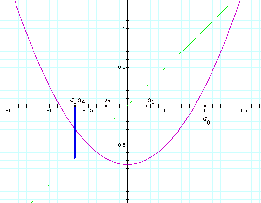
If you extend this table far enough, you'll see the iterates slowly approach the number –0.5. The iterates are above or below –0.5, but they get closer and closer to –0.5. In summary, when the initial value is a0 = 1.0, the iterates stay small, and, in particular, they approach –0.5.

It helps to see what's going on graphically. In the diagram above, the graph y = x2 – 0.75 of our function is drawn in magenta. Also, to help us see the iterates, the line y = x is drawn in green. Then the values a0, a1, a2, a3, and a4 are shown grapically, starting with our first value of a0, namely, 1.0. To find an+1 from an, follow the vertical blue line to the graph of the function (the magenta curve), then follow the horizontal red line across to the diagonal green line y = x, then follow another vertical blue line back to the x-axis. Notice how close a4 is to a2, but just a little to the right. The iterate a5 isn't shown on the graph, but it would be a little to the left of a3. If the rest of the iterates were shown, you would see a rectangular spiral in blue and red closing in on the point where the magenta curve and the green line intersect, that is, at the point (–0.5,–0.5). Thus, the iterates approach –0.5.
With different initial values, different things can happen to the iterates. Let's take this time a0 = 2.0. Here's the table of iterates.
| a0 = | 2.0, |
| a1 = | f(2.0) = 4.02 – 0.75 = 3.25 |
| a2 = | f(3.25) = 3.252 – 0.75 = 9.8125 |
| a3 = | f(9.8125) = 9.81252 – 0.75 = 95.535 |
| a4 = | f(95.535) = 95.5352 – 0.75 = 9126.2 |
| a5 = | f(9126.2) = (9126.2)2 – 0.75 = 83287819.2 |
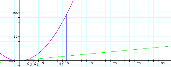
Here's the graph of the iterates starting with the initial value a0 = 2.0. The graph is colored in the same way, but it's drawn to a different scale. This time, the iterates run off to infinity; they don't remain small.
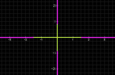
Thus, what happens in the long run depends on the initial value a0. It's easy to show that if the initial value a0 is greater than 1.5, then the iterates run off to infinity, like they did when a0 was 2.0. Also, when the initial value a0 is less than –1.5, then, since after one iteration a1 is greater than 1.5, the iterates go off to infinity. With more work, you can show that if –1.5 < a0 < 1.5, then the iterates approach –0.5, like they did when a0 was 1.0. The remaining two initial values, namely 1.5 and –1.5, have all their iterates equal to 1.5. So the set of real numbers is partitioned into two parts, the closed interval [–1.5,1.5] of initial values whose iterates remain bounded, and the rest of the real numbers whose iterates do not remain bounded but approach infinity. This is shown graphically below. The real line is partitioned into the two sets with the interval [–1.5,1.5] drawn in light yellow, the rest in pink. We'll call the set of initial values whose iterates remain bounded the filled-in Julia set, or simply the Julia set for short. Thus, the light yellow set is the real Julia set for the function f(x) = x2 – 0.75.

Complex numbers. We'll continue studying this same function, but extend our comprehension to complex numbers. For background on complex numbers, see Dave's Short Course on Complex Numbers.
When we go to complex functions, we'll use z as the independent variable to emphasize that we're working with complex numbers. So, we write our sample function as f(z) = z2 – 0.75.
What happens when the initial value a0 is a complex number instead of a real number? Let's take a0 to be the imaginary number i for an example. The table of iterates of this function looks like this.
| a0 = | i, |
| a1 = | f(i) = i2 – 0.75 = –1 – 0.75 = –1.75 |
Ah, let's stop there. We have the real number –1.75, and we know from the analysis above that it's iterates go to infinity since –1.75 is not in the range from –1.5 to 1.5.
Let's try another imaginary number, say 0.5i.
| a0 = | 0.5i, |
| a1 = | f(0.5i) = (0.5i)2 – 0.75 = –0.25 – 0.75 = –1 |
Again, we can stop because we found that the iterate a1, which equals –1, does lie in the range from –1.5 to 1.5. Therefore, it's iterates converge.
We could try other pure imaginary numbers ci where c is a real number. We would find that the iterates are bounded whenever –c2 – 0.75 lies in the range from –1.5 to 1.5. A little algebra shows that occurs when c2 is less than or equal to 0.75, that is, when ci is between 0.866i and –0.766i. Therefore, on the complex axis, we should color the imaginary numbers between o.866i and –0.866i light yellow, the others pink.
We have begun to explore the complex Julia set for this function, but only just begun. Let's try another complex number for a0.
Let's take a0 to be the complex number 1/3 + 5i/9. We'll get this table of iterates.
| a0 = | 1/3 + 5i/9 = 0.3333 + .5556i |
| a1 = | f(1/3 + 5i/9) = (1/3 + 5i/9)2 – 0.75 = –0.9475 + 0.3704i |
| a2 = | f(–0.9475 + 0.3704i) = 0.0106 + 0.7019i |
| a3 = | f(0.0106 + 0.7019i) = –1.2424 + 0.0149i |
| a4 = | f(–1.2424 + 0.0149i) = 0.7933 - 0.0371i |
| a5 = | f(0.7933 - 0.0371i) = –0.1221 + 0.5891i |
Well, it's unclear what's going to happen in the long run from looking at just these first five iterates. It looks like it's time to turn the computation over to a computer.
What we need a computer to do is try lots of different initial complex values a0. For each value, iterate the function until it's clear whether the iterates approach infinity. It isn't hard to find how far away from 0 an value has to be in order that further iterates run away to infinity, but it's hard to conclude that all the iterates remain bounded. So what's done here is look at a limited number of iterates. If one gets far enough from 0, then we know the iterates will approach infinity. But if all remain sufficiently close to 0, then we won't draw any certain conclusion.
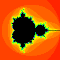
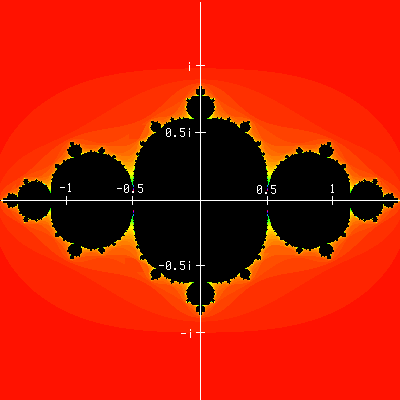
Just below the result of that computation for our function f(z) = z2 – 0.75. The image shows the part of the complex plane including numbers z = x + iy where both x and y are between ±1.5 is shown.) The black part of the plane indicates that the iterates did not get far from 0, so for an initial value a0 in that region, all the iterates (probably) remain bounded. The black region includes the parts of the axes in the previous image that were drawn in light yellow.
Most of the rest of the plane is colored red shading to some other colors. In this colored region of the plane, the iterates soon left toward infinity. Different colors indicate how soon, with red being quite quickly, yellow taking longer, and green, blue, and magenta taking much longer. This colored region includes the parts of the axes in the previous image that were drawn in pink.
That finishes our example of iterating a function. This was a quadratic function gave an interesting Julia set. Linear functions like f(z) = 3z + 5 don't yield interesting partitions of the complex plane, but quadratic and higher degree polynomials do as do other nonlinear functions.
A natural source of iterated functions comes from the approximation of roots of functions by Newton's method.
 Consider a whole family of functions parameterized by a variable. Although any family of functions
can be studied, we'll look at the most studied family, that being the family of quadratic polynomials
f(x) = x2 - µ, where µ is a complex parameter. As µ
varies, the Julia set will vary on the complex plane. Some of these Julia sets will be connected,
and some will be disconnected, and so this character of the Julia sets will partition the
µ-parameter plane into two parts. Those values of µ for which the Julia set is connected
is called the Mandelbrot set in the parameter plane. The boundary between the Mandelbrot set and
its complement is often called the Mandelbrot separator curve. The Mandelbrot set is the black shape
in the picture. This is the portion of the plane where x varies from -1 to 2 and y
varies between -1.5 and 1.5. There are some surprising details in this image, and it's well worth exploring.
The bulk of the Mandelbrot set is the black cardioid. (A cardioid is a heart-shaped figure). It's
studded with circles all around its boundary.
 Here's a magnification of the region of the
circle on top of the cardioid. Note that this circle as well as the other circles you can see are
also studded with circles. There are infinitely many circles on the cardioid, each of those circles
has infinitely many circles on them, and on and on ad infinitum. That makes for a lot of
circles!
 The green figure is a Julia set with the parameter µ taken from the center of the circle on top
of the cardioid.
If you look close, you'll see the strands of dark blue above the circle under discussion. So, what's going on up there? Here's a blowup of that portion of the figure.
Aha! There's something black up near the top of the picture. What's that?
 It's another cardioid with associated circles! Not exactly the same, but close. In fact, there are
lots of these tiny little clusters. You can find them along the filaments connecting everything
together.
© 1994, 1995, 2003.
Email: 
These pages are located at http://aleph0.clarku.edu/~djoyce/julia/