
Any characters can be used to classify species and reconstruct a phylogenetic tree of species, but some are more useful than others. If a species depends on a character for its continued survival, that character will not change as any mutations of it will be eliminated. Call such characters essential. And most visible characters are essential for the species. This means that if we choose essential characters, any differences should count as very significant. There are, however, some difficulties with considering essential characters. If one species evolves by changing an essential characteristic, whatever ecological forces supported that change may also apply to other species, and that could lead to parallel evolution. Thus, differences or similarities in essential characters are very relevant to the reconstruction of the general shape of the phylogenetic tree, but they really can't be used to determine the relative lengths of the lines within the tree. Some species have been stable for millions of years. Others evolve very fast.
Irrelevant mutations. We could, on the other hand, consider nonessential characters. Changes in nonessential characters are effected by mutations, mutations that we can call irrelevant. The rate of change of irrelevant mutations should be fairly uniform among species, especially among species that are fairly closely related. Unfortunately, if a character really doesn't matter, it should be very difficult to perceive the value of that character in a species.
Much of the genome sequence of an organism is irrelevant. For example, there are 64 (43) different codons for 20 amino acids. Some amino acids are coded by up to four different codons. For these multiply coded amino acids, typically the third nucleotide can take any of the four possible values. In other words, a mutation in this third nucleotide is irrelevant. The DNA can mutate at this site and the resulting protein doesn't change.
By concentrating on irrelevant mutations, not only can the shape of the phylogenetic tree be reconstructed, but the relative lengths of the lines within the phylogenetic tree can also be estimated.
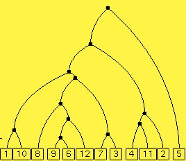
Controls. The diagram above shows a phylogenetic tree. You can ask for a new tree and change the number of extant species as before. These are the controls in the yellow portion of the control panel; they determine the random selection of a model phylogenetic tree.
The pink portion of the control panel allows you to control mutations. There are a number of characters being tracked, 40 by default. Each character has a number of alternate values, 4 by default. You can also set the mutation rate, 100 by default. A value of 100 means that the mutation rate for each character is 100/1000 mutations per unit time interval. That means that along a line in the model tree of length 1 unit, there will be about 1 mutation per 10 characters. If you hike the mutation rate up too far (like 10000), you'll see that it looks like the values of the characters are completely unrelated among the various species. If you set the mutation rate down to 1, you may not see any mutations at all (but any you see will be very important in reconstructing the tree).
The side window of gene sequences. In a resizable side window, you can see the characters of each of the the extant species in a column, the rows being the different characters. The alternative values are shown in different colors. For instance, if all the species have the same color in a row, then that character hasn't mutated, or else they've all mutated to the same new value. (Incidentally, all characters start out with the same character value, denoted red in the window.) If in some row, two of the species show one green, but three show red, then that's some indication that the two species are more closely related to each other than they are to the other three, while the other three species are more closely related to each other then they are to the first two. Of course, that's a statistical indication. The variance in all the characters should be taken into consideration to reconstruct the tree.
Mutations as a measure of time. Let's concentrate on one character to begin with. Our first questions are: What is the probability p(t) that the character has some value at the beginning of a time interval of length t as it does at the end? What is the probability q(t) that the character has one value at the beginning of a time interval of length t but a different value at the end of the interval?
Suppose that there are m different possible alternate values, and suppose that the mutation rate is r mutations per unit time interval.
Some statistical analyisis (which we'll skip) gives us the answers to these questions.

Note that initially, when t = 0, p(0) is 1, while q(0) is 0 since there are no mutations in no time. Also, as t approaches infinity, p(t) and q(t) both approach 1/m, which means that in the long run, each of the m alternative values are equally probable.
Now let's assume that there are n different characters, not just one. Then E(t), the expected number of characters that are not the same at the end of a time interval of length t as they were at the beginning, is n(m –1) q(t), that is,

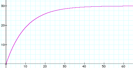
Here's the graph of that function when there are m = 4 alternate values for each character, there are n = 40 characters, and the mutation rate is r = 0.1. Time t is shown on the horizontal axis, while the vertical axis gives y, the expected number of character differences.

Note that when t gets large, the expected number of character differences approaches 30.
We can take the inverse function of y = E(t), that is, turn this graph around, to give us an estimate for time t in terms of the observed number of character differences. Let g denote the inverse function. Then

 The base of the logarithm function here is e.
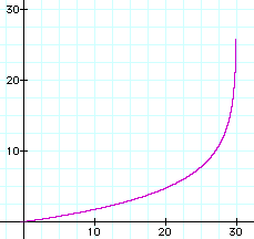
The graph of t = g(y) is shown to the right with the same parameter values m = 4, n = 40, and r = 0.1.
Note that as the number of expected differences approaches 30, the corresponding time approaches infinity. The observed number of differences may be near the expected number, but it's usually more or
less. So the observed number of differences could easily be greater than 30. Should that happen, the best conclusion to make is that the time is very great, but can't be estimated.
It would be prudent not to estimate the time when the number of differences is slightly less than 30, too.
Next page: distances between species.
Previous page: introduction.
Table of contents: http://aleph0.clarku.edu/~djoyce/java/Phyltree.
David E. Joyce

Department of Mathematics and Computer Science
Clark University
November, 2002